Swipr - Fast.ai and CNNs
Finally we can consider creating the image classification model. The jupyter notebook that was used for this process can be found here on GitHub.
DataLoader
The first thing the creation of a PyTorch model requires is the creation of a DataLoader, which is a neat structure for handling the data we want to go over and what their labels should be. It loads x’s (inputs) and maps them to y’s (outputs).
In previous DL experiments on this blog, we’ve used text/nlp loaders, and more complicated custom loader for handling audio data, but this time since we have an image problem, we don’t have to do anything complicated, and can use the best and easiest part fast.ai.
Label CSV
The label CSV, in this particular use-case of an image classifier, is a file that contains the locations of our images that we want to analyze and their appropriate output classification.
We have a very simple desired output - binary classification of either YES or NO, representing a potential LIKE or PASS on Tinder.
At this point we actually have yet to properly curate these classifications for our images, having just grouped the downloaded files into a few different buckets like GENERAL_NO, TOO_YOUNG, etc.
We’ll do that now.
One benefit of the SQLite file we created earlier that stored the picture locations with their respective pre-filtered status codes is that we can use that same file to construct our desired training set and their classifications on the fly.
Runtime Generation of Labels.csv
First we should define what we want from our model. We downloaded a bunch of pictures, ran face detection over it, asked it for how many people were in the picture, and what their ages and genders were. Let’s codify some rules now:
FAIL_ON_MALE = True # We set this to true because we aren't interested in the nn learning to say yes to men.
MAX_PEOPLE = 1 # if set to zero, there is no upper limit on people in the picture.
MIN_PEOPLE = 1 # We set this to 1 because we want the NN to reject pictures of food, beaches, etc
MIN_AGE = 0 # if set to zero, there is no lower limit on the age of people in the picture. See above as to why.
MAX_AGE = 0 # if set to zero, there is no upper limit on the age of people in the picture.
The thing we do is construct what we want a NO or a YES to be with respect to our downloaded and pre-filtered images:
WITH_BABY = "with_baby"
TOO_YOUNG = "too_young"
TOO_OLD = "too_old"
PURIKURA = "purikura"
GENERAL_NO = "general_no"
OK = "OK"
Tinder_DUDES = "Tinder_dudes"
Tinder_GIRLS = "Tinder_girls"

MainDirs = {
    WITH_BABY: "insta/with_baby/",
    TOO_YOUNG: "insta/too_young/",
    TOO_OLD: "insta/too_old/",
    PURIKURA: "insta/purikura/",
    GENERAL_NO: "insta/no/",
    OK: "insta/ok/",
    Tinder_DUDES: "Tinder/dudes",
    Tinder_GIRLS: "Tinder/girls",
}

YesLabels = [OK]
NoLabels = [Tinder_DUDES, Tinder_GIRLS, WITH_BABY, TOO_YOUNG, TOO_OLD, PURIKURA, GENERAL_NO]
Next we ask our SQLite file for all images that weren’t unloadable. That is, every image that wasn’t corrupted or something:
def Filter():
    conn, cursor = GetSql()
    q = "SELECT path, label, ages, num_people, male_present FROM pics WHERE label NOT IN (?);"
    yeses = []
    nos = []
    for row in cursor.execute(q, (FAIL_INVALID_INT, )):
        p = row[0]
        if _Filter(row):
            yeses.append(p)
        else:
            nos.append(p)
    return yeses, nos
Then we put our pre-filter to work assembling our YesLabels. Just because the picture was from the OK path of our Instagram directories doesn’t mean we want to blindly accept it. Remember, no beaches and no food:
def _Filter(row, verbose=False):
    # Get the path of our consideration
    p = row[0]

    # Check that path isn't in our unconditional 'no' set
    for nopath in [MainDirs[x] for x in NoLabels]:
        if p.startswith(nopath):
            return False

    # Check that the label doesn't immediately disqualify from consideration
    label = row[1]
    if label in [FAIL_NOFACE_INT, FAIL_ROTATEDNOCHANGED_INT]:
        return False

    # check number of people
    num_people = row[3]
    if MAX_PEOPLE > 0 and num_people > MAX_PEOPLE:
        return False

    # Check that there are no males
    male_present = row[4]
    if FAIL_ON_MALE and male_present:
        return False

    # Check ages
    age_str = row[2].split(',')
    ages = []
    for x in age_str:
        try:
            a = int(x)
            ages.append(a)
        except:
            continue
    if MIN_AGE > 0:
        min_passed = all([x >= MIN_AGE for x in ages])
        if not min_passed:
            return False
    if MAX_AGE > 0:
        max_passed = all([x <= MAX_AGE for x in ages])
        if not max_passed:
            return False

    return True
The output of all this is a list of image paths separated into legitimate YES images, and the rest of them are NO:
y,n = Filter()
len(n)
201573

len(yeses)
47777
It’s a heavily skewed dataset, but such is life on Instagram: Roughly 50,000 images from our 300,000 collection are ok to learn what a Tinder LIKE should be, and the rest are all what a Tinder PASS should be.
Recall that passes will include the whole shebang: Pictures of dogs, beaches, food, men, and women who just aren’t our type.
We can now assemble our labels.csv on the fly using these modular creation methods:
def MakeCSV(cname, yeses, nos):
    with open(PATH/cname, 'w', newline='', encoding="utf8") as csvfile:

        resolved = PATH.resolve()

        # get a csv writer with some defaults
        cwriter = csv.writer(csvfile, delimiter=',', quotechar='|', quoting=csv.QUOTE_MINIMAL)

        # Write the header
        cwriter.writerow(["path", "label"])

        # write the nos
        for p in nos:
            cwriter.writerow([os.path.join(resolved, p), "NO"])

        # write the yesses
        for p in yeses:
            cwriter.writerow([os.path.join(resolved, p), "YES"])

    return PATH/cname
label_csv = MakeCSV("labels.csv", y, n)
Validation Set
fast.ai offers an easy way to divide a set of labels into a training set and a validation set via the get_cv_indexes method, which we will use here:
n = len(list(open(label_csv)))-1
val_idxs = get_cv_idxs(n)
The method randomly chooses some percentage of the total dataset to become the validation set. In our case, we got about 50,000 images for the validation set:
len(val_idxs)
50991
Architecture
It’s now time to make perhaps the most major choice regarding our model yet. What will our architecture be? Should we build something from scratch or use a pre-existing arch? What should our initial weights be?
Although these are heavy questions, we will make our decision with somewhat less gravitas. As the adage for deep learning projects goes, if you have an image classification problem, throw ResNet at it and see if it works.
For no reason in particular, instead of ResNet, we’ll use FAIR’s ResNext50. Why? Because. It’s like ResNet, but not. It comes pre-installed with the fast.ai libraries and is pre-trained on weights from ImageNet.
This is particularly useful to us because ImageNet is really good for real-world photographs, and shouldn’t require much additional training. That is, we don’t have to spend time teaching it what a “human” is, and can instead essentially jump right into teaching it what is worth swiping left or right on.
Size
One of the image-specific settings we need to set is what the dimension of the images we’re going to hand into the model should be. Although named needlessly similar to the BatchSize parameter, they aren’t related concepts.
Images need to be square for the current state-of-the-art convnet algos to do their magic, and they can’t be especially large squares at that.
We’ll be taking a lot of cues from Jeremey’s fast.ai introductory lesson about Dogs vs Cats since it matches our problem of binary image classification well.
There he chose a dimension size of 224 x 224. Images beyond that size will be resized and cropped if necessary, and images below that size will be padded out to make up for it.
Batch Size
This is one of our most magical hyperparameters, second only in importance to the mythical learning rate.
As a quick overview, the batch size is the number of observations (in our case, discrete images) that will be loaded onto the GPU at once. These images are all operated upon together and used to discern the gradient to descend. This is the data the gradient part of gradient descent is calculated from.
In theory, the bigger a batch a size the more granular and accurate the resulting gradient is, but it is neither practical (due to GPU memory limitations) nor even necessarily useful to try to maximize this batch size parameter. In some cases it may even be harmful, contributing in part to why the batch size is considered magical.
If you’re following along with Jeremy’s courses, you may hear him refer to a minibatch - that refers to a BatchSize-sized list of data being handed to the neural net for gradient calculations. In essence:
Image[] minibatch = new Image[BatchSize];
Our batch size here, like in the Cats vs Dogs lesson, will be 24, but you are encouraged to play around and measure your results.
Transforms
We keep saying fast.ai has splendid support for you if your use-case involves going over images and our next task is a small testament to that.
fast.ai supports the notion of data augmentation during training, which is a way to avoid overfitting by slightly adjusting the data handed in while attempting to keep the meaning of the data unchanged. In our case, we want to run some transformations over our training images:
tfms = tfms_from_model(arch, sz, aug_tfms=transforms_side_on, max_zoom=1.1)
This function, supplied by the fast.ai library, produces a list of other functions which will transform each image in various ways.
Basically, we’ll flip the images horizontally and zoom in up to an additional 10%.
The idea behind this step is that a picture of, for example, a cat, is a cat even if it’s zoomed in, or even if it’s facing the other direction. Cat’s are not unidirectional objects so we want our NN to avoid fitting to that particular aspect.
The same idea applies for Tinder pictures.
Back to the DataLoader
We’re going to combine everything from above into a custom dataloader creation function:
def get_data(size, batchSize):
    tfms = tfms_from_model(arch, size, aug_tfms=transforms_side_on, max_zoom=1.1)
    data = ImageClassifierData.from_csv(PATH, PATH, label_csv, val_idxs=val_idxs, tfms=tfms, bs=bs)
    return data if size > 300 else data.resize(340, "tmp")
This is taken straight from the Dogs vs Cats lesson. It resizes each picture in the dataset and stores everything into tmp.
Our dataloader can be instantiated like so:
data = get_data(sz, bs)
The paths are for the train and validation sets, because images are expected to be relative to the current working directory. We pass in the same path for both fields, along with the val_idxs, tfms, and bs from earlier.
We can see the relative sizes of our datasets like so:
len(data.trn_ds), len(data.val_ds)
(203966, 50991)
We can check our classes:
len(data.classes), data.classes
(2, ['NO', 'YES'])
Notably this means that index 0 is NO and index 1 is YES. This is good information for later.
Learner Object
The last step of our model creation odyssey is to instantiate a learner object and call fit on it:
learn = ConvLearner.pretrained(arch, data, precompute=False)
We ask for a pretrained learner because we want to use the weights from ResNext50, and we want precompute=False because we’re not trying to fine-tune the last layers, we want to spend some effort really substantially updating all the intermediate weights.
Of course like every other time we start this process with the learning rate finder:
learn.lr_find()
learn.sched.plot_lr()
The usual graphs:
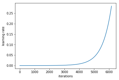
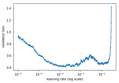
We want to find the learning ate that seems most likely to give us the greatest ability to descend, while also leading us to the widest area of our data, spatially speaking. From the graph, although a learning rate of 1e^-0.5 leads to a good curve, 1e-4 leads us to a similar depth while giving us a wider valley.
We’ll choose 1e-4 first and see where we go from there:
learn.fit(1e-4, 3, cycle_len=1, cycle_mult=2)
After a very long time, we got the following results:
| epoch | trn_loss | val_loss | accuracy |
|---|---|---|---|
| 0 | 0.399513 | 0.392782 | 0.819912 |
| 1 | 0.403108 | 0.390016 | 0.822238 |
| 2 | 0.393089 | 0.39024 | 0.822318 |
| 3 | 0.388752 | 0.38785 | 0.824343 |
| 4 | 0.399516 | 0.384942 | 0.825968 |
ImageNet weights are already good, so we start right on off with a 0.38 validation loss.
Next, we tried the following:
learn.set_data(get_data(229,bs))
learn.freeze()
Primarily we freeze everything but the last layer and see if we get better results. We also try with a slightly higher learning rate of 1e-3.
We end up with the following:
learn.fit(1e-3, 3, cycle_len=1, cycle_mult=2)
| epoch | trn_loss | val_loss | accuracy |
|---|---|---|---|
| 0 | 0.372923 | 0.365708 | 0.832845 |
| 1 | 0.359612 | 0.364647 | 0.832565 |
| 2 | 0.382324 | 0.368091 | 0.832244 |
We tried a number of other possibilities, involving both starting at different learning rates, or using the same object and changing the learning rate, and also resizing
It looks like we’re topping out around a 0.36 validation loss meaning a roughly 83% accuracy.
Training these variants totaled around 10 hours.
Other Considerations
Potential other model architectures included integrating the InsightFace and DFace steps, creating something from scratch, or otherwise better integrating the Tinder pictures, because we just labeled them all as NO by default.
Needless to say, we went the lazy route, because an 83% accuracy is already pretty good.
Moving on
In the next post we’ll discuss moving the model to our CPU-only server and constructing a small framework to interact with it.
Next Section - Swipr Script Service